Convert CML data

This module provides functions to convert CML xarray data into other formats such as GeoDataFrames.

cml = open_cml_sample()

Convert sublinks to GeoDataFrame

When a CML has multiple sublinks, they share the same geometry. To visualize them distinctly on a map, we offset each sublink perpendicularly to the link direction using the normal vector of the line. Sublinks alternate on each side of the original link, spreading outward.

Warning

The perpendicular offset is applied in degrees of longitude/latitude. Near the equator, 1° of longitude ≈ 1° of latitude ≈ 111 km, so the default offset of 2e-4° ≈ 20 m. At higher latitudes, degrees of longitude shrink (by a factor of cos(latitude)), so the same offset in degrees will correspond to a different physical distance.

cml_df = cml_df.dropna(subset=["site_0_lat", "site_0_lon", "site_1_lat", "site_1_lon", "frequency"], how="any")
cml_df.head(2)

	cml_id	sublink_id	frequency	site_0_lat	site_0_lon	site_1_lat	site_1_lon	transmitter	length
0	4.056847N-9.738556E	0_0	12765.0	4.060028	9.726194	4.053667	9.750917	0.0	2834.0
1	4.056847N-9.738556E	0_1	13031.0	4.060028	9.726194	4.053667	9.750917	1.0	2834.0

We define the direction vector \(\mathbf{v}\) for each sublink as the difference in coordinates: \[\mathbf{v} = (\Delta \text{lon}, \Delta \text{lat}) = (\text{lon}_1 - \text{lon}_0, \text{lat}_1 - \text{lat}_0)\]

As you move away from the equator, the distance represented by one degree of longitude shrinks. To make our direction vector \(\mathbf{v}\) meaningful in a local Cartesian-like space, we need to scale the longitudinal component (\(\Delta \text{lon}\)) by the cosine of the latitude:

\[\Delta \text{lon}_{\text{scaled}} = \Delta \text{lon} \cdot \cos(\phi)\]

where \(\phi\) is the latitude (converted to radians in your code). This ensures that a “step” in the x-direction is physically comparable to a “step” in the y-direction, regardless of where the link is located on Earth.

To make the sublinks visually distinct, we calculate a normal vector (\(\mathbf{n}\)) that is perpendicular to the link’s direction vector (\(\mathbf{v}\)).

If our direction vector is \(\mathbf{v} = (v_x, v_y)\), we can find a perpendicular vector by swapping the components and negating one: \[\mathbf{n} = (-v_y, v_x)\]

You can check that this is perpendicular because the dot product \(\mathbf{v} \cdot \mathbf{n} = v_x(-v_y) + v_y(v_x) = 0\).

However, this normal vector \(\mathbf{n}\) might have any length. To control the offset distance precisely, we need a unit normal vector (\(\mathbf{\hat{n}}\)) with a length of 1: \[\mathbf{\hat{n}} = \frac{\mathbf{n}}{||\mathbf{n}||} = \frac{(-v_y, v_x)}{\sqrt{(-v_y)^2 + v_x^2}}\]

Because we calculated the normal vector \(\mathbf{n}\) in a Cartesian-like space where the x-axis was compressed by \(\cos(\phi)\), its longitudinal component \(n_x\) is currently in those scaled units. To use this as a coordinate offset in degrees of longitude, we must “unscale” it:

\[n_{x, \text{degrees}} = \frac{n_{x, \text{scaled}}}{\cos(\phi)}\]

This brings the vector component back to the original degree units so it can be added directly to the latitude and longitude coordinates.

To calculate the offset for each sublink, we will determine a magnitude based on the sublink’s position relative to the main link:

1. Relative Numbering: Each sublink is assigned an index \(i\).
2. Alternating Direction: We assign a sign \(s \in \{-1, 1\}\) to ensure sublinks are distributed on both sides of the main link path: \[s = (i \pmod 2) \cdot 2 - 1\]
3. Magnitude: The total offset \(M\) is calculated by multiplying the base offset \(O\) (approx. 20m) by the pairing factor \(\lfloor i/2 \rfloor\) and the alternating sign: \[M = O \cdot \lfloor i/2 \rfloor \cdot s\]

This creates a spreading effect where sublinks are placed at increasing distances from the center, alternating in direction for better visualization. The center of the link is left empty to be able to plot the link.

Finally, we shift the coordinates of both the start point (\(P_0\)) and the end point (\(P_1\)) of the sublink by the calculated magnitude (\(M\)) along the unit normal vector (\(\mathbf{\hat{n}}\)) to obtain the new geometry coordinates:

\[P_{0, \text{new}} = P_0 + M \cdot \mathbf{\hat{n}}\] \[P_{1, \text{new}} = P_1 + M \cdot \mathbf{\hat{n}}\]

Warning

The offset is applied only to the coordinates of the lines that form the GeoDataFrame geometry, not to the original site coordinate columns stored in the metadata. This distinction is crucial to preserve the original data, ensuring that you can easily perform backward conversion from a GeoDataFrame back to the original xarray format later.

---

source

convert_sublinks_to_gdf

def convert_sublinks_to_gdf(
    cml:xarray.core.dataarray.DataArray | xarray.core.dataset.Dataset, # CML data
    only_meta:bool=True, # The GeoDataFrame will only contain metadata
    offset:float=0.0002, # Perpendicular offset in degrees (2e-4 ~ 20m in the equator) in order to avoid overlap in visualization
)->GeoDataFrame:

Convert CML to a GeoDataFrame assuming EPSG:4326 projection

convert_sublinks_to_gdf(cml).plot()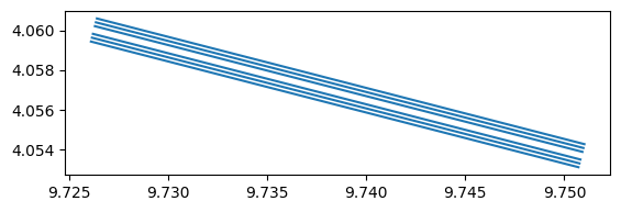

convert_sublinks_to_gdf(cml, only_meta=False).head(2)

	cml_id	sublink_id	time	frequency	site_0_lat	site_0_lon	site_1_lat	site_1_lon	transmitter	length	geometry	rsl_avg	tsl_avg	rsl_min	tsl_min	rsl_max	tsl_max
0	4.056847N-9.738556E	0_0	2019-07-01 00:05:00	12765.0	4.060028	9.726194	4.053667	9.750917	0.0	2834.0	LINESTRING (9.72614 4.05983, 9.75087 4.05347)	-43.3	13.0	-43.4	13.0	-43.1	13.0
1	4.056847N-9.738556E	0_0	2019-07-01 00:20:00	12765.0	4.060028	9.726194	4.053667	9.750917	0.0	2834.0	LINESTRING (9.72614 4.05983, 9.75087 4.05347)	-43.2	13.0	-43.3	13.0	-43.1	13.0