cml, baseline = open_cml_sample(), open_cml_sample("baseline")Path Average Rain Rate Estimation
This module contains methods for estimating rain rates from path-integrated attenuation (PIA). Currently, we compute the time-mean total precipitation rate as defined by ECMWF, using
tprate as the variable name for simplicity. Note that while ECMWF uses units of \(m·s^{-1}\), we may use different units such as \(mm·h^{-1}\).
k-R law for Network Management System (NMS) min/max sampling
The rain rate (\(R\)) can be estimated from the specific attenuation (\(k\)) expressed in \(dB·km^{-1}\) using an exponential law known as the k-R relationship: \[ k = aR^b \] where \(a\) and \(b\) are parameters that depend on the frequency, polarisation and drop size distribution (DSD). However, the available attenuation is the Path Integrated Attenuation: \[ PIA = \int_0^L k(l) \, dl \] where \(L\) is the length of the link. We are interested in the path-averaged rain rate \(\bar{R}\), and the above relationship can be approximated as:
\[ PIA = \int_0^L k(l) \, dl = \int_0^L a R(l)^b \, dl \stackrel{b \approx 1}{=} a \bar{R}^b L \] The further \(b\) deviates from 1, the more imprecise this relationship becomes. If attenuation sampling is not instantaneous (e.g., 15 minutes), PIA is also time-averaged; thus \(\bar{R}\) becomes the time-mean path-averaged precipitation rate.
Considering that the sample data is located in Douala, and that the \(a\) and \(b\) coefficients are dependent on the DSD, which varies by region, we will first develop the coefficients estimated by Alcoba (2019).
alcoba_2019_africa_coefs
def alcoba_2019_africa_coefs(

)->Dataset:
k-R relationship coefficients for Africa from Alcoba (2019).
alcoba_2019_africa_coefs().to_dataframe()| a | b | |
|---|---|---|
| frequency | ||
| 7000 | 0.000197 | 1.8540 |
| 8500 | 0.006600 | 1.2897 |
| 11000 | 0.019500 | 1.1951 |
| 11500 | 0.023000 | 1.1775 |
| 13000 | 0.034700 | 1.1333 |
| 14500 | 0.047300 | 1.1022 |
| 15000 | 0.051700 | 1.0943 |
| 18000 | 0.078100 | 1.0654 |
| 19000 | 0.087300 | 1.0600 |
| 22000 | 0.117100 | 1.0471 |
| 23000 | 0.128100 | 1.0428 |
Warning
While different coefficient assignment algorithms are available (see below), they all based on some form of nearest value. If your frequencies differ significantly from those listed, you may need to use a downscaling algorithm (such as interpolation) to generate coefficients for your specific frequencies before estimating rainfall.
In many scenarios, NMS only save the min and max values for the sampling interval. Thus rain rate has to be estimated from those values. Overeem et al. (2013), developped an algorithm that computes time mean path averaged rain rate for 15 minute interval sampling based only on minimum and máximum values. The algorith asumes that the TSL is constant for each time. Thus máximum and mínimum attenuations are computed as follows:
\[ A_{min} = (TSL - RSL_{min}) - baseline \]
\[ A_{max} = (TSL - RSL_{max}) - baseline \]
Then rain rate is estimated as follows.
\[ \bar{R}_{min | max} = a \left(\frac{A_{min|max} - WAA}{L}\right)^b H(A_{min|max} - WAA) \quad \]
\(H(x)\) is the Heaviside step function, defined as:
\[ H(x) = \begin{cases} 0 & \text{if } x \leq 0 \\ 1 & \text{if } x > 0 \end{cases} \]
The baseline and WAA have already been developed in other submodules, meaning that PIA can easily be obtained. Therefore, to maintain the modular approach, the focus will be on obtaining the \(\bar{R}\) from the PIA. \[ \bar{R}_{min | max} = a \left(\frac{PIA_{min|max}}{L}\right)^b H(PIA_{min|max}) \quad \] Where PIA is defined as: \[ PIA_{min|max} = A_{min|max} - WAA \]
Finally we can complute \(\bar{R}\) as a weighted average of \(\bar{R}_{max}\) and \(\bar{R}_{min}\): \[ \bar{R} = \alpha \bar{R}_{max} + (1 - \alpha) \bar{R}_{min} \quad \]
Overeem et al. (2013) estimated and optimal value of \(\alpha=0.33\) by calibrating the model using 12 days of data from the Netherlands. We use this value as a reasonable default; however, it should be calibrated for each specific region and deployment.
get_overeem_et_al_2013_min_max_nms_tprate
def get_overeem_et_al_2013_min_max_nms_tprate(
    pia:Dataset, # ds containing the minimum and maximum Path Integrated Attenuations (PIA)
    cfs:Dataset, # ds containing `a` and `b`, k-R law coefficients as variable and `frequency` as dim
    cfs_assign_method:str='nearest', # xr.sel method used to map the pia frequencies to the cfs freqs
    alpha:float=0.3, # weighting factor between max and min sampling rain rates
    name_min:str='pia_min', # Name of the variable containing minimum PIA
    name_max:str='pia_max', # Name of the variable containing maximum PIA
)->Dataset:
Compute the rain rate using the Overeem et al. (2013) min/max sampling approach.
tprate = get_overeem_et_al_2013_min_max_nms_tprate(pia, alcoba_2019_africa_coefs())
tprate
<xarray.Dataset> Size: 18MB
Dimensions: (cml_id: 126, sublink_id: 6, time: 2964)
Coordinates: (10)
Data variables:
tprate (cml_id, sublink_id, time) float64 18MB 0.0 0.0 0.0 ... 0.0 0.0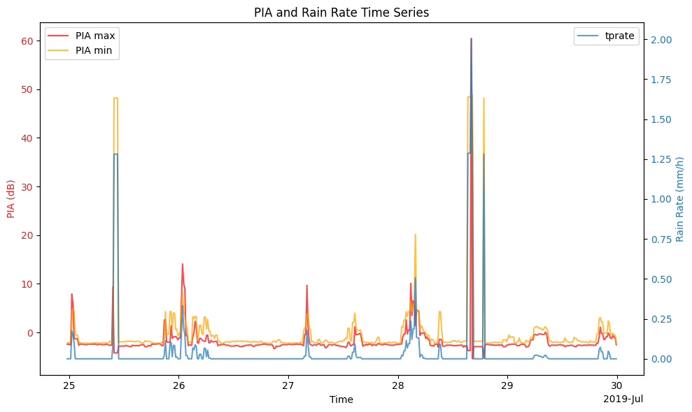
References
- Alcoba Kait, M. 2019. A contribution to rainfall observation in Africa from polarimetric weather radar and commercial microwave links. Ph.D. dissertation, Université Paul Sabatier – Toulouse III, 202 pages. https://tel-02955598 (accessed 2025‑11‑21).
- Overeem, A., H. Leijnse, and R. Uijlenhoet, 2013: Country-wide rainfall maps from cellular communication networks. Proceedings of the National Academy of Sciences, 110, 2741–2745, doi:10.1073/pnas.1217961110.
- Chwala, C., and H. Kunstmann, 2019: Commercial Microwave Link Networks for rainfall observation: Assessment of the current status and future challenges. WIREs Water, 6, doi:10.1002/wat2.1337.